Battle of the MEMs: Burg vs. Shannon for Directional Wave Spectrum Reconstruction

Introduction

Wave buoys are the most common devices used to measure ocean waves. Oceanographers and engineers worldwide rely on wave buoys to monitor sea state conditions, validate numerical models, and ensure the safety of maritime operations. However, a persistent challenge with buoy data is that they can generally resolve only a handful of Fourier coefficients: typically just the first and second harmonics ( $a_1$ , $b_1$ , $a_2$ , $b_2$ ). This makes it tricky to estimate the full directional distribution $D(\theta)$ , which describes how wave energy is spread across directions.

Maximum Entropy Methods (MEM) are among the most widely used approaches for reconstructing the directional spectrum from this limited information. Yet, in practice, the world of MEM can be surprisingly confusing: there are two different methods (and several numerical methods), the naming differs across sources, etc. A common pitfall in the literature is that some authors often benchmark against only one MEM, overlooking the fact that the two methods produce fundamentally different results.

In this post, I’ve tested both MEM approaches hands-on, and I’ll share not only the main findings but also step-by-step implementations so you can try these methods yourself. Please note that this is just my understanding based on my experience working with these methods. I’m not an expert on MEM, so if you spot any mistakes or have further insights, I’d be glad to hear them!

The Two Methods

1. MEM-I (based on Burg’s entropy definition)

MEM-I, developed by Lygre and Krogstad (1986), is based on maximizing Burg’s entropy, defined as:

S_\mathrm{Burg} = -\int_0^{2\pi} \ln D(\theta)\, \frac{d\theta}{2\pi}

This approach treats the directional distribution as an autoregressive (AR) process. It solves the Yule-Walker equations to find coefficients $\phi_1$ and $\phi_2$ , then constructs the directional distribution using this formula:

D(\theta) = \dfrac{\sigma^2}{2\pi|1 - \phi_1 e^{-i\theta} - \phi_2 e^{-2i\theta}|^2}

Here, $\sigma^2$ is the “error variance” (representing residual energy not explained by the AR model), while $\phi_1$ and $\phi_2$ are the autoregressive (AR) coefficients of the model. The terms $c_1$ and $c_2$ correspond to the complex first and second Fourier coefficients extracted from the buoy data (i.e., $c_n = a_n + i b_n$ for $n=1,2$ ).

The beauty of this method is that it’s entirely closed-form—no iteration required. Here’s the core implementation in Python:

def directional_mem_burg(theta, a1, b1, a2, b2):
    """
    Compute directional distribution using Burg's Maximum Entropy Method.
    Based on Lygre and Krogstad (1986).
    """
    # Complex Fourier coefficients
    c1 = a1 + 1j * b1
    c2 = a2 + 1j * b2

    # Solve Yule-Walker equations
    denom = 1 - np.abs(c1)**2
    if denom < 1e-6:
        phi2 = 0
        phi1 = c1
    else:
        phi2 = (c2 - c1**2) / denom
        phi1 = c1 - phi2 * np.conj(c1)

    # Error variance
    sigma2 = 1 - (phi1 * np.conj(c1) + phi2 * np.conj(c2)).real

    # Compute directional distribution
    e_it = np.exp(-1j * theta)
    e_2it = np.exp(-2j * theta)
    poly = 1 - phi1 * e_it - phi2 * e_2it

    D = sigma2 / (2 * np.pi * np.abs(poly)**2)
    return D

The main advantage? Speed. You can process thousands of spectra per second, making it ideal for real-time applications.

2. MEM-II (based on Shannon’s entropy definition)

MEM-II takes a different approach: it finds the distribution that maximizes Shannon entropy while matching the measured Fourier coefficients exactly. The solution has this exponential form:

$D(\theta) = \dfrac{\exp(\lambda_1\cos\theta + \lambda_2\sin\theta + \lambda_3\cos2\theta + \lambda_4\sin2\theta)}{Z}$

where $Z$ is the normalisation factor (the integral of the unnormalised exponential over all directions) that ensures the distribution integrates to 1, making it a valid density function. The Lagrange multipliers $\lambda_1$ , $\lambda_2$ , $\lambda_3$ , and $\lambda_4$ are found by solving a system of constraint equations iteratively.

The relationship between the Lagrange multipliers and Fourier coefficients is established through constraint equations: the multipliers are chosen such that the Fourier coefficients computed from the resulting distribution $D(\theta)$ exactly match the measured coefficients $(a_1, b_1, a_2, b_2)$ from the buoy data. Specifically, $\lambda_1$ and $\lambda_2$ control the first harmonic (matching $a_1$ and $b_1$ ), while $\lambda_3$ and $\lambda_4$ control the second harmonic (matching $a_2$ and $b_2$ ).

Here’s a simplified implementation:

def directional_mem_shannon(theta, a1, b1, a2, b2):
    """Compute directional distribution using Shannon's Maximum Entropy Method (MEM-II)"""

    theta_array = np.asarray(theta)
    
    # Define the constraint equations
    def constraints(lambdas):
        l1, l2, l3, l4 = lambdas
        
        # Integration points
        theta_int = np.linspace(0, 2*np.pi, 360)
        
        # Unnormalized distribution
        exp_arg = (l1*np.cos(theta_int) + l2*np.sin(theta_int) + 
                   l3*np.cos(2*theta_int) + l4*np.sin(2*theta_int))
        
        # Avoid overflow
        exp_arg = exp_arg - np.max(exp_arg)
        D_unnorm = np.exp(exp_arg)
        
        # Normalization constant
        Z = np.trapz(D_unnorm, theta_int)
        
        # Normalized distribution
        D_norm = D_unnorm / Z
        
        # Compute Fourier coefficients
        a1_est = np.trapz(D_norm * np.cos(theta_int), theta_int)
        b1_est = np.trapz(D_norm * np.sin(theta_int), theta_int)
        a2_est = np.trapz(D_norm * np.cos(2*theta_int), theta_int)
        b2_est = np.trapz(D_norm * np.sin(2*theta_int), theta_int)
        
        return [a1_est - a1, b1_est - b1, a2_est - a2, b2_est - b2]
    
    # Initial guess
    lambda0 = [2*a1, 2*b1, 2*a2, 2*b2]
    
    try:
        lambdas_opt = fsolve(constraints, lambda0)
        l1, l2, l3, l4 = lambdas_opt
    except:
        # Fallback to minimization
        def objective(lambdas):
            return np.sum(np.array(constraints(lambdas))**2)
        res = minimize(objective, lambda0, method='Nelder-Mead')
        l1, l2, l3, l4 = res.x
    
    # Compute D(θ) at requested angles
    exp_arg = (l1*np.cos(theta_array) + l2*np.sin(theta_array) + 
               l3*np.cos(2*theta_array) + l4*np.sin(2*theta_array))
    exp_arg = exp_arg - np.max(exp_arg) # Stability
    D_unnorm = np.exp(exp_arg)
    
    # Normalize
    theta_int = np.linspace(0, 2*np.pi, 360)
    exp_arg_int = (l1*np.cos(theta_int) + l2*np.sin(theta_int) + 
                   l3*np.cos(2*theta_int) + l4*np.sin(2*theta_int))
    exp_arg_int = exp_arg_int - np.max(exp_arg_int)
    Z = np.trapz(np.exp(exp_arg_int), theta_int)
    
    return D_unnorm / Z

This method is a bit slower because it requires iterative solving, but as we’ll see, it produces significantly more accurate results.

Performance Comparison

To rigorously test these methods, I generated a library of synthetic directional distributions using the Donelan et al. (1985) $\operatorname{sech}^2$ spreading function, defined as:

$D(\theta) = \dfrac{1}{2}\beta\, \operatorname{sech}^2\!\big(\beta(\theta - \theta_m)\big)$

where $\beta$ controls the narrowness/broadness of the directional distribution.

This model is widely used because it closely matches real ocean wave directional spreading.

I tested six cases covering different scenarios:

Unimodal Narrow: Sharp peak (β=20), like swell from a distant storm
Unimodal Broad: Wide spread (β=2), like locally generated wind sea
Bimodal Far (Equal): Two equal peaks 90° apart
Bimodal Close (Equal): Two equal peaks 20° apart
Bimodal Far (Unequal): Two peaks of different energy, far apart
Bimodal Close (Unequal): Two unequal peaks close together

Here’s what the comparison looks like:

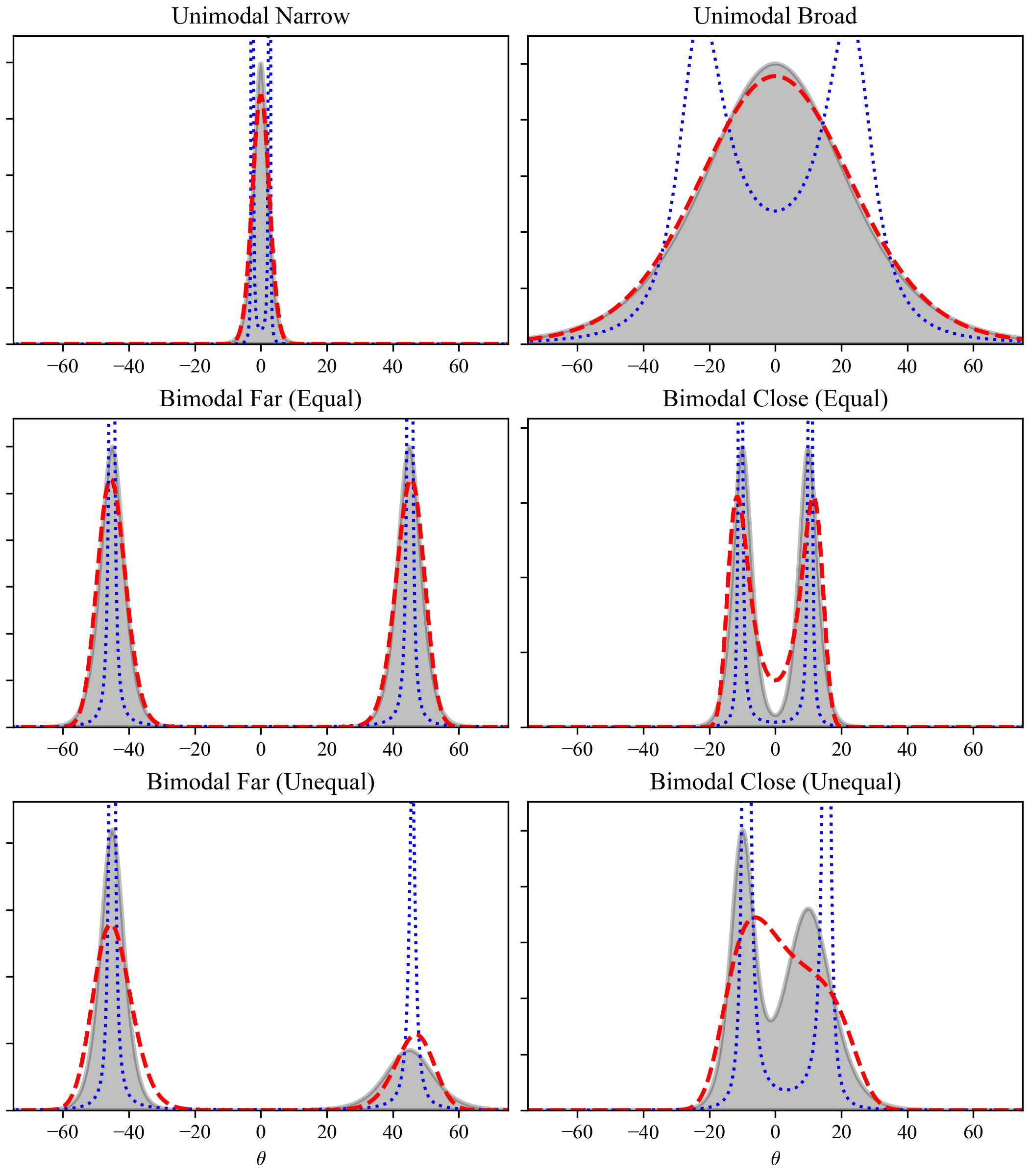
Comparison of MEM-I and MEM-II across six test cases

Six-panel comparison showing true directional distributions (black filled) versus reconstructions using MEM-I (blue dotted) and MEM-II (red dashed).

The visual differences are striking. MEM-I performs reasonably well on simple unimodal distributions but fails catastrophically on bimodal cases, often creating spurious peaks or missing peaks entirely. MEM-II generally reproduces the true distribution with high accuracy across most cases, but it does have limitations: when the two peaks in a bimodal distribution are very close together, MEM-II tends to merge them into a single broader peak and cannot fully resolve both modes. In all other cases, MEM-II closely matches the true distribution.

Quantitative Results

To quantify this, I ran both methods on 100 randomly generated distributions (mix of unimodal and bimodal) and computed three error metrics:

RMSE (Root Mean Square Error):
$\mathrm{RMSE} = \sqrt{ \frac{1}{N} \sum_{i=1}^{N} \left[ D_{\text{est}}(\theta_i) - D_{\text{true}}(\theta_i) \right]^2 }$
Measures the average squared difference between the estimated and true distributions.
KL Divergence (Kullback–Leibler Divergence):
$D_{\mathrm{KL}} = \sum_{i=1}^{N} D_{\text{true}}(\theta_i) \log \left( \frac{D_{\text{true}}(\theta_i)}{D_{\text{est}}(\theta_i)} \right)$
Quantifies the information loss when using the estimate instead of the true distribution (lower = better).
Fourier Error (Fourier Coefficient Error):
$\varepsilon_{\mathrm{Fourier}} = \sqrt{ (a_1 - \tilde{a}_1)^2 + (b_1 - \tilde{b}_1)^2 + (a_2 - \tilde{a}_2)^2 + (b_2 - \tilde{b}_2)^2}$
Gives the Euclidean distance between the estimated and true Fourier coefficients.

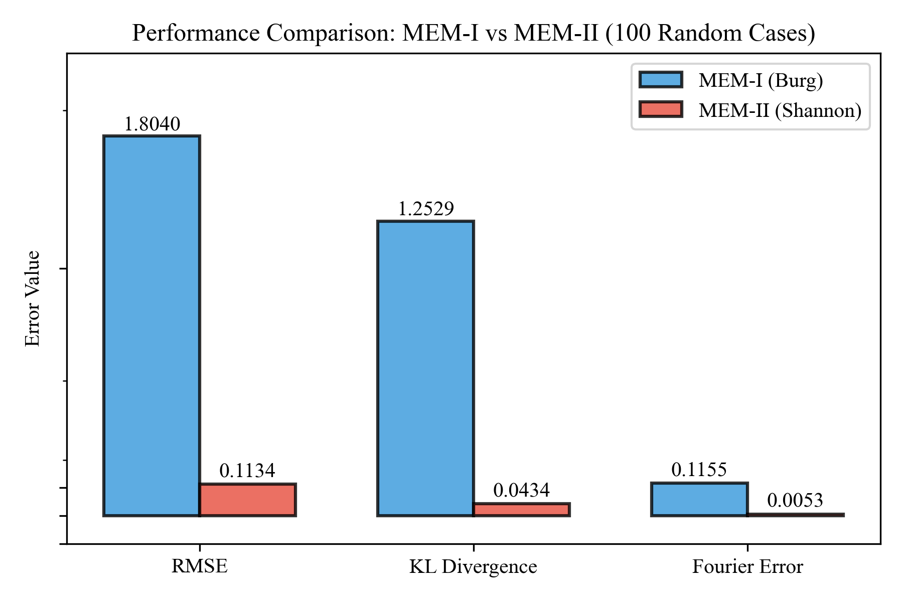
Performance metrics comparison between MEM-I and MEM-II

Average error metrics from 100 random test cases. MEM-II (red) consistently outperforms MEM-I (blue) across all metrics.

The numbers speak for themselves:

Metric	MEM-I (Burg)	MEM-II (Shannon)	Improvement
RMSE	1.898 ± 0.983	0.124 ± 0.067	15× better
KL Divergence	1.317 ± 0.429	0.051 ± 0.072	26× better
Fourier Coefficient Error	0.119 ± 0.170	0.005 ± 0.007	24× better

MEM-II is not just marginally better, it’s an order of magnitude more accurate.

Computational Cost

On my machine (Macbook M4 Max), processing times for a single spectrum:

MEM-I: ~0.1 ms (10k spectra/second)
MEM-II: ~5 ms (200 spectra/second)

Even MEM-II is fast enough for most applications. If you’re processing millions of spectra, consider vectorising or using parallel processing.

Conclusion

In summary: MEM-II outperforms MEM-I for all cases except when two peaks are very close together—only then does MEM-II struggle to resolve both. For most practical scenarios, MEM-II is much more accurate.

The choice between MEM-I and MEM-II comes down to the accuracy-speed tradeoff. For most oceanographic research, I recommend using MEM-II as the default. The 15–26 times improvement in accuracy is substantial, and the computational cost is negligible for modern systems.

Use MEM-I only when you have a specific reason: real-time constraints, known-simple spectra, or resource limitations. But be aware of its limitations, particularly with bimodal distributions—which are common in the real ocean when swell and wind sea coexist.

The full implementation with all test cases is available in the Jupyter notebook if you want to experiment with your own data.

References

Lygre, A., & Krogstad, H. E. (1986). Maximum Entropy Estimation of the Directional Distribution in Ocean Wave Spectra. J. Phys. Oceanogr., 16(12), 2052–2060. doi: 10.1175/1520-0485(1986)016<2052:MEEOTD>2.0.CO;2
Hashimoto, N., Nagai, T., & Asai, T. (1995). Extension of the Maximum Entropy Principle Method for Directional Wave Spectrum Estimation. In Coastal Engineering 1994, 272–286. ASCE. doi: 10.1061/9780784400890.019
Simanesew, A. W., & Krogstad, H. E. (2018). Bimodality of Directional Distributions in Ocean Wave Spectra: A Comparison of Data-Adaptive Estimation Techniques. J. Atmos. Ocean. Technol., 35(2), 365–384. doi: 10.1175/JTECH-D-17-0007.1
Christie, D. C. (2024). Efficient estimation of directional wave buoy spectra using a reformulated Maximum Shannon Entropy Method: Analysis and comparisons for coastal wave datasets. Appl. Ocean Res., 142, 103830. doi: 10.1016/j.apor.2023.103830
Donelan, M. A., Hamilton, J., & Hui, W. H. (1985). Directional Spectra of Wind-Generated Waves. Phil. Trans. R. Soc. Lond. A, 315(1534), 509–562. doi: 10.1098/rsta.1985.0054