Spectrum reconstruction from IOWAGA partitions
D.S. Peláez-Zapata
July 23, 2019D.S. Peláez-Zapata
July 23, 2019Sometimes is quite useful to have the information of the frequency-direction wave spectrum instead of only the bulk wave parameters. But unfortunately this information is scarce. In this post we present a simple methodology to reconstruct the directional wave spectrum using the bulk parameters from the spectrum partitions taken from the IOWAGA dataset.
As usual, the first thing to do is import the essential Python packages, in this
case, we only need NumPy,
matplolib and
netCDF4.
import numpy as np
import datetime as dt
import matplotlib.pyplot as plt
import matplotlib.colors as mcolors
import netCDF4 as nc
import os
%matplotlib inline
The JONSWAP (Joint North Sea Wave Project) spectrum is a representation of the wave energy distribution in terms of the frequency and the direction, for a given sea state. It was originally developed by Hasselmann et al. in 1973. The current form of the JONSWAP spectral shape can be written as:
\[\begin{aligned} S(f) &= \frac{\alpha g^2}{(2\pi)^4 f^5} \exp \left( -\beta_0 \left(\frac{f_p}{f}\right)^4 \right) \gamma^{\delta} \\ \delta &= \exp\left( -\frac{(f-f_p)^2}{2(\sigma_0 f_p)^2} \right) \\ \sigma_0 &= \left\{ \begin{array}{lr} 0.07 & : f < f_p \\ 0.09 & : f \ge f_p \end{array} \right. \end{aligned}\]where $\alpha=8.1 \times 10^{-3}$, $\beta_0=5/3$, and $f_p$ is the peak frequency. Well, the frequency distribution is more or less well-know but the directional distribution is somehow more complex. In this case we are going to use the one proposed by Donelan and colleagues:
\[\begin{aligned} D(f,\theta) &= 0.5 \beta \mathrm{sech}^2 \beta (\theta - \theta_m(f)) \\ \beta &= \left\{ \begin{array}{lcr} 2.61 (f/f_p)^{1.3} & : & 0.56 < f/f_p < 0.95 \\ 2.28 (f/f_p)^{-1.3} & : & 0.95 < f/f_p < 1.60 \\ 10^p & : & f/f_p > 1.60 \end{array} \right. \\ p &= -0.4 + 0.8393 \cdot e^{-0.567 \ln (f/f_p)^2} \end{aligned}\]Well, we are ready to code these functions in Python. First, we are going to
write a function called jonswap which will receive three arguments:
frequencies array, significant wave height, peak period, and shape factor, and
it will return an array containing the spectral variance density with the same
size of the frequencies array:
# jonswap spectrum
def jonswap(frqs, Hs, Tp, gamma=3.3):
    """Returns the JONSWAP spectrum for a given Hs, Tp and frequency array"""

    # constants
    fp = 1./Tp
    alpha, beta, g = 8.1E-3, 5./4., 9.8

    # it should be vectorized!
    S = np.zeros_like(frqs)
    for i, f in enumerate(frqs):
        if f == 0.:
            S[i] = 0.
        else:
            num = alpha * (g**2)
            den = ((2*np.pi)**4) * f**5
            pm = (num / den) * np.exp(-beta * (fp/f)**4)
            sigma = 0.07 if f <= fp else 0.09
            r = np.exp(-(f - fp)**2 / (2.*(sigma**2)*(fp**2)))
            S[i] = pm * gamma**r

    # scale spectrum with zero-order moment
    m0 = np.trapz(S, x=frqs)
    return (S / m0) * (Hs**2 /16)
Now, for the directional distribution we can construct another function, this
time, the arguments that will be passed are: the frequencies array, the
directions array (in degrees), and again, the bulk parameters, including the
mean wave direction. Additionally, we can include the kind of distribution
function we want, for example, sech2 for Donelan et al. distribution, and
cos2s for the classical $\cos^{2s}\theta$ distribution, passing the $s$
parameter as an argument:
# directional wave spectrum
def directional_wave_spectrum(frqs, dirs, Hs, Tp, mdir, func="cos2s", s=1):
    """Returns the directional wave spectrum"""

    # frequency spectrum from jonswap
    S = jonswap(frqs, Hs=Hs, Tp=Tp, gamma=3.3)

    # direction arrays
    dir2 = (dirs - mdir) % 360 # <-- centered in the mean direction
    dir3 = dirs - 180          # <-- wrapped between -180 and 180

    # cos2s
    if func == "cos2s":
        #
        D = (2. / np.pi) * np.cos((dirs - mdir)*np.pi/180.)**(2*s)
        D[np.logical_and(dir2>90, dir2<270)] = 0.
        E = S[None,:] * D[:,None]

    # sech2
    if func == "sech2":
        #
        ffp = frqs*Tp
        beta = np.ones(len(frqs))*1.24
        beta[np.logical_and(ffp>=0.56, ffp<0.95)] = 2.61 * ffp[np.logical_and(ffp>=0.56, ffp<0.95)]**(1.3)
        beta[np.logical_and(ffp>=0.95, ffp<1.60)] = 2.28 * ffp[np.logical_and(ffp>=0.95, ffp<1.60)]**(-1.3)
        E = S[None,:] * (beta[None,:] / 2) * np.cosh(beta[None,:] * (dir3[:,None])*np.pi/180.)**(-2)
        #
        ixd = np.argsort(((dir3 + mdir) % 360))
        E = E[ixd,:]

    # scale spectrum with zero-order moment
    m0 = np.abs(np.trapz(np.trapz(E, x=np.radians(dirs), axis=0), x=frqs))
    return (E / m0) * (Hs**2 / 16)
Now, let’s code a small function to plot the directional wave spectrum.
# plot wave spectrum
def plot_wave_spectrum(frqs, dirs, E, ax=None, label_angle=-45):
    """Polar representation of a directional wave spectrum"""

    if dirs[-1] != 360.:
        E_copy = E.copy()
        dirs = np.append(dirs, 360)
        E = np.zeros((len(dirs), len(frqs)))
        E[:-1,:] = E_copy
        E[-1,:] = E_copy[0,:]

    Fx = frqs[None,:] * np.cos(dirs[:,None]*np.pi/180)
    Fy = frqs[None,:] * np.sin(dirs[:,None]*np.pi/180)

    if not ax:
        fig, ax = plt.subplots(1,1, figsize=(5,5), dpi=120)

    colors = ["#FFFFFF", "#01DFA5", "#FE642E", "#08298A", "#01A9DB"]
    cmap = mcolors.LinearSegmentedColormap.from_list('cmap', colors, N=1024)

    smin, smax= -1., 2.
    norm = mcolors.LogNorm(vmin=10**smin, vmax=10**smax)

    pc = ax.pcolormesh(Fx, Fy, E, cmap=cmap, norm=norm)
    cf = ax.contour(Fx, Fy, E, np.array([0.25, 0.5, 0.75, 1.0])*E.max(), colors="k")

    ax.text(0.50, 0.95, "N", transform=ax.transAxes, ha="center", va="center")
    ax.text(0.95, 0.50, "E", transform=ax.transAxes, ha="center", va="center")
    ax.text(0.50, 0.05, "S", transform=ax.transAxes, ha="center", va="center")
    ax.text(0.05, 0.50, "W", transform=ax.transAxes, ha="center", va="center")
    ax.set_xticklabels([])
    ax.set_yticklabels([])
    ax.set_ylabel("$f \, \mathrm{ [Hz]}$")

    fmax, fstep = 0.5, 0.1
    ax.set_xlim((-0.4, 0.4))
    ax.set_ylim((-0.4, 0.4))

    ticks = np.append(np.arange(-fmax, 0, fstep), np.arange(0, fmax+fstep, fstep)[1:])
    for radii in ticks[ticks > 0]:
        circle = plt.Circle((0,0), radii, color="0.5", linestyle="dashed", fill=False)
        ax.add_artist(circle)
        ax.text(radii*np.cos(np.radians(label_angle)),
                radii*np.sin(np.radians(label_angle)),
                f"{radii:.1f}")
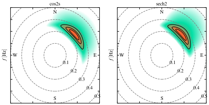
A good way to test our function is plotting the two directional distribution side-by-side, moreover it is useful to see the differences:
frqs = np.linspace(0,1,256)
dirs = np.arange(360)
E_sech2 = directional_wave_spectrum(frqs, dirs, Hs=2, Tp=4, mdir=45, func="sech2")
E_cos2s = directional_wave_spectrum(frqs, dirs, Hs=2, Tp=4, mdir=45, func="cos2s", s=4)

fig, (ax1, ax2) = plt.subplots(1, 2, figsize=(7,3.5), dpi=120)
plot_wave_spectrum(frqs, dirs, E_cos2s, ax=ax1)
plot_wave_spectrum(frqs, dirs, E_sech2, ax=ax2)
ax1.set_title("cos2s")
ax2.set_title("sech2")
# download file from ifremer ftp server
def download_from_ftp(filename):
    """Copy file from FTP to local directory"""

    local_path = "/Volumes/Boyas/iowaga/"

    with ftplib.FTP("ftp.ifremer.fr") as ftp:

        # login the ftp
        ftp.login()
        ftp.cwd("ifremer/ww3/HINDCAST/")

        # create local folder if it does not exist
        folder = os.path.join(local_path, os.path.split(filename)[0])
        if not os.path.exists(folder):
            os.makedirs(folder)

        print(f"Downloading from FTP: {filename}")
        with open(os.path.join(local_path, filename), "wb") as f:
            cmd = f"RETR {filename}"
            try:
                ftp.retrbinary(cmd, f.write)
                return True
            except:
                print("File couldn't be downloaded")
                return False
# load dataset
def load_dataset(year, month, region="GLOBAL", wind_source="ECMWF"):
    """Returns all the netcdf datasets por the specific region"""

    local_path = "/Volumes/Boyas/iowaga/"
    basename = f"{region}/{year}_{wind_source}/partitions"

    if region == "GLOBAL":
        grid = "30M"
        rcode = "GLOB"
    else:
        grid = "10M"

    dic = {}
    list_of_variables = ["phs", "pdir", "ptp"]
    for variable in list_of_variables:
        for partition in range(6):

            # create filename
            parameter = f"{variable}{partition}"
            filename = f"{basename}/WW3-{rcode}-{grid}_{year}{month:02d}_{parameter}.nc"

            # check if local filename exist
            local_filename = os.path.join(local_path, filename)
            if os.path.exists(local_filename):
                dataset = nc.Dataset(local_filename, "r")
            #
            # if not, download it from ftp server
            else:
                result = download_from_ftp(filename)
                if result:
                    dataset = nc.Dataset(local_filename, "r")

            # store in a dictionary
            dic[parameter] = dataset

    return dic
# extract data in a specific point
def extract_point(dic, date, lon=-96.6245, lat=24.6028):
    """Extract the partition parameters in a specific point"""

    results = {}
    for parameter, dataset in dic.items():

        # choose the interest variables
        time = nc.num2date(dataset["time"][:].data, dataset["time"].units)
        glat = dataset["latitude"][:]
        glon = dataset["longitude"][:]

        # find the indices of the specific point
        ixtime = np.argmin(abs(time - date))
        ixlat = np.argmin(abs(glat - lat))
        ixlon = np.argmin(abs(glon - lon))

        # load the variables in a point
        value = np.float32(dataset[parameter][ixtime, ixlat, ixlon])
        results[parameter] = value

    # save lon, lat and time
    results["lon"] = glon[ixlon]
    results["lat"] = glat[ixlat]
    results["time"] = time[ixtime]

    return results
# construct spectrum
def construct_spectrum(results):
    """Return spectrum for the parameters passed in results"""

    # create spectrum using a sech function
    frqs = np.arange(0.01, 1, 0.01)
    dirs = np.arange(360)
    E = np.zeros((len(dirs), len(frqs)))
    #
    for partition in range(6):
        Hs = results[f"phs{partition}"]
        Tp = results[f"ptp{partition}"]
        pdir = (270-results[f"pdir{partition}"]) % 360
        #
        if Hs != 0:
            E += directional_wave_spectrum(frqs, dirs, Hs, Tp, pdir, func="sech2")

    return frqs, dirs, E
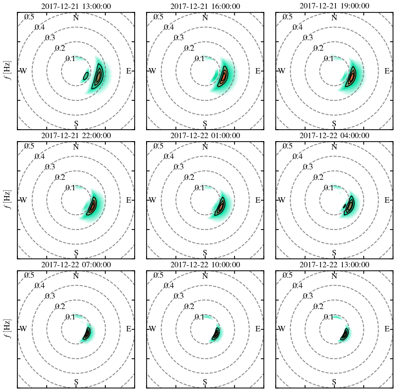
# define date and location
date = dt.datetime(2017, 12, 21, 13, 0)
lon, lat =-116.83, 31.82

# create canvas
fig, ax = plt.subplots(3, 3, figsize=(7,7), dpi=120)
fig.subplots_adjust(top=.95, bottom=.05, left=.05, right=.95, wspace=.1, hspace=.1)
ax = np.ravel(ax)

# loop for each panel (nine in total)
for i in range(9):
    #
    results = extract_point(dic, date, lon=lon, lat=lat)
    frqs, dirs, E = construct_spectrum(results)
    #
    if i in [2,5,8]:
        plot_wave_spectrum(frqs, dirs, E, ax=ax[i], label_angle=135)
    else:
        plot_wave_spectrum(frqs, dirs, E, ax=ax[i], label_angle=135)

    # set title
    title = date.strftime("%Y-%m-%d %H:%M:%S")
    ax[i].set_title(title)

    # tune up axes
    if i not in [6,7,8]:
        ax[i].set_xlabel("")
        ax[i].set_xticklabels([''])
    #
    if i not in [0,3,6]:
        ax[i].set_ylabel("")
        ax[i].set_yticklabels([''])

    # next spectrum
    date += dt.timedelta(hours=3)